Introduction
aphid is an R package for the development and application of hidden Markov models and profile HMMs for biological sequence analysis. It contains functions for multiple and pairwise sequence alignment, model construction and parameter optimization, file import/export, implementation of the forward, backward and Viterbi algorithms for conditional sequence probabilities, tree-based sequence weighting, and sequence simulation. The package has a wide variety of uses including database searching, gene-finding and annotation, phylogenetic analysis and sequence classification.
Hidden Markov models (HMMs) underlie many of the most important tasks in computational biology, including multiple sequence alignment, genome annotation, and increasingly, sequence database searching. Originally developed for speech recognition algorithms, their application to the field of molecular biology has increased dramatically since advances in computational capacity have enabled full probabilistic analysis in place of heuristic approximations. Pioneering this transition are two groups lead by Anders Krogh and Sean Eddy, whose respective software packages SAM and HMMER have underpinned HMM-based bioinformatic analysis for over two decades.
Here, we present the aphid package for analysis with profile hidden Markov models in the R environment (R Core Team 2017). The package contains functions for developing, plotting, importing and exporting both standard and profile HMMs, as well as implementations of the forward, backward and Viterbi algorithms for computing full and optimal conditional sequence probabilities. The package also features a multiple sequence alignment tool that produces high quality alignments via profile HMM training.
Dependencies
The aphid package is designed to work in conjunction with the “DNAbin” and “AAbin” object types produced using the ape package (Paradis, Claude, and Strimmer 2004; Paradis 2012). These object types, in which sequences are represented in a bit-level coding scheme, are preferred over standard character-type sequences for maximizing memory and speed efficiency. While we recommend using ape alongside aphid, it is not a requisite and as such is listed in the “Suggests” rather than “Imports” section of the package description. Indeed, any sequence of standard ASCII characters is supported, making aphid suitable for other applications outside of biological sequence analysis. However, it should be noted that if DNA and/or amino acid sequences are input as character vectors, the functions may not recognize the ambiguity codes and therefore are not guaranteed to treat them appropriately.
To maximize speed, the low-level dynamic programming functions (including the forward, backward, Viterbi, and maximum a posteriori algorithms) are written in C++ linking to the Rcpp package (Eddelbuettel and Francois 2011). R versions of these functions are also maintained for the purposes of debugging, experimentation and code interpretation. This package also relies on the openssl package (Ooms 2016) for sequence and alignment comparisons using the MD5 hash algorithm.
Classes
Two primary object classes, “HMM” (hidden Markov model) and “PHMM” (profile hidden Markov model) are generated using the aphid functions deriveHMM and derivePHMM, respectively. These objects are lists consisting of emission and transition probability matrices (elements named “E” and “A”), and non-mandatory elements that may include vectors of background emission and transition probabilities (“qe” and “qa”, respectively) and other model metadata including “name”, “description”, “size” (the number of modules in the model), and “alphabet” (the set of symbols/residues emitted by the model). Objects of class “DPA” (dynamic programming array) are also generated by the Viterbi and forward/backward functions. These are predominantly created for the purposes of succinct console-printing.
Functions
HMMs and PHMMs are explained in more detail throughout the following sections using aphid package functions to demonstrate their utility. The examples are borrowed from Durbin et al (1998), to which users are encouraged to refer for a more in-depth explanation on the theory and application of these models. Book chapter numbers are provided wherever possible for ease of reference.
Hidden Markov Models
A hidden Markov model is a hypothetical data-generating mechanism for a sequence or set of sequences. It is depicted by a network of states each emitting symbols from a finite alphabet according to a set of emission probabilities, whose values are specific to each state. The states are traversed by an interconnecting set of transition probabilities, that include the probability of remaining in any given state and those of transitioning to each of the other connected states.
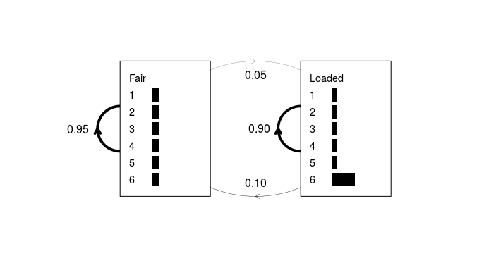
An example of a simple HMM is given in Durbin et al (1998) chapter 3.2. An imaginary casino has two dice, one fair and one weighted. The fair dice emits residues from the alphabet {1, 2, 3, 4, 5, 6} with equal probabilities (1⁄6 for each residue). The probability of rolling a “6” with the loaded dice is 0.5, while that of each of the other five residues is 0.1. If the dealer has the fair dice, he may secretly switch to the loaded dice with a probability of 0.05 after each roll, leaving a 95% chance that he will retain the fair dice. Alternatively, if he has the loaded dice, he will switch back to the fair dice with a probability of 0.1, or more likely, retain the loaded dice with a probability of 0.9.
This example can be represented by a simple two-state hidden Markov model. The following code manually builds and plots the “HMM” object.
library("aphid")
states <- c("Begin", "Fair", "Loaded")
residues <- paste(1:6)
### Define transition probability matrix A
A <- matrix(c(0, 0, 0, 0.99, 0.95, 0.1, 0.01, 0.05, 0.9), nrow = 3)
dimnames(A) <- list(from = states, to = states)
### Define emission probability matrix E
E <- matrix(c(rep(1/6, 6), rep(1/10, 5), 1/2), nrow = 2, byrow = TRUE)
dimnames(E) <- list(states = states[-1], residues = residues)
### Create the HMM object
x <- structure(list(A = A, E = E), class = "HMM")
### Plot the model
plot(x, textexp = 1.5)
### Optionally add the transition probabilities as text
text(x = 0.02, y = 0.5, labels = "0.95")
text(x = 0.51, y = 0.5, labels = "0.90")
text(x = 0.5, y = 0.9, labels = "0.05")
text(x = 0.5, y = 0.1, labels = "0.10")
 Figure 1: A simple hidden Markov model for the dishonest casino
example. The plot.HMM method depicts the transition probabilities as
weighted lines, and emission probabilities as horizontal grey bars. No
begin/end state is modeled in this example; however, this can be
achieved by entering non-zero probabilities in the first row and column
of the transition matrix and passing “begin = TRUE” to
 plot.HMM.
For a sequence of observed rolls, we can establish the most likely sequence of hidden states (including when the dice-switching most likely occurred) using the Viterbi algorithm. In the example given in Durbin et al (1998) chapter 3.2, the observed sequence of 300 rolls is:
##  31511624644664424531132163116415213362514454363165
##  66265666666511664531326512456366646316366631623264
##  55236266666625151631222555441666566563564324364131
##  51346514635341112641462625335636616366646623253441
##  36616611632525624622552652522664353533362331216253
##  64414432335163243633665562566662632666612355245242
Some observable clusters of 6’s suggest that the loaded dice made an appearance at some stage, but when did the dice-switching occur? In the following code, the Viterbi algorithm is used to find the most likely sequence of hidden states given the model.
data(casino)
### The actual path is stored in the names attribute of the sequence
actual <- c("F", "L")[match(names(casino), c("Fair", "Loaded"))]
### Find the predicted path
vit1 <- Viterbi(x, casino)
predicted <- c("F", "L")[vit1$path + 1]
### Note the path element of the output Viterbi object is an integer vector
### the addition of 1 to the path converts from C/C++ to R's indexing style
Comparing the predicted path with the actual hidden sequence, the Viterbi algorithm wasn’t far off:
##  Actual     FFFFFFFFFFFFFFFFFFFFFFFFFFFFFFFFFFFFFFFFFFFFFLLLLL
##  Predicted  FFFFFFFFFFFFFFFFFFFFFFFFFFFFFFFFFFFFFFFFFFFFFFFFLL
##
##  Actual     LLLLLLLLLLLLLLLLFFFFFFFFFFFFLLLLLLLLLLLLLLLLFFFLLL
##  Predicted  LLLLLLLLLLLLLLLLFFFFFFFFFFFFLLLLLLLLLLLLLLLLLLLLLL
##
##  Actual     LLLLLLLLLLLFFFFFFFFFFFFFFFFFLLLLLLLLLLLLLFFFFFFFFF
##  Predicted  LLLLLLLLLLLLFFFFFFFFFFFFFFFFFFFFFFFFFFFFFFFFFFFFFF
##
##  Actual     FFFFFFFFFFFFFFFFFFFFFFFFFFFFLLLLLLLLLLFFFFFFFFFFFF
##  Predicted  FFFFFFFFFFFFFFFFFFFFFFFFFFFFFLLLLLLLLLLLLLFFFFFFFF
##
##  Actual     FFFFFFFFFFFFFFFFFFFFFFFFFFFFFFFFFFFFFFFFFFFFFFFFFF
##  Predicted  FFFFFFFFFFFFFFFFFFFFFFFFFFFFFFFFFFFFFFFFFFFFFFFFFF
##
##  Actual     FFFFFFFFFFFFFFFFFLLLLLLLLLLLLLLLLLLLLLLFFFFFFFFFFF
##  Predicted  FFFFFFFFFFFFFFFFFFFFLLLLLLLLLLLLLLLLLLLFFFFFFFFFFF
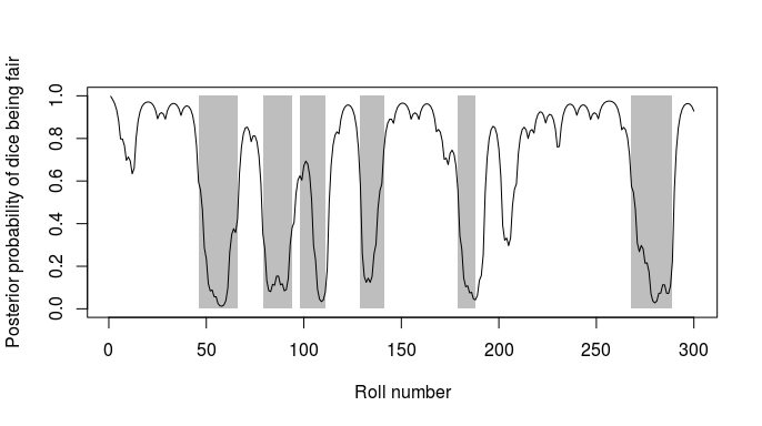
We can also calculate the full and posterior probabilities of the
sequence given the model using the forward and/or backward
algorithms:
casino.post <- posterior(x, casino)
plot(1:300, seq(0, 1, length.out = 300), type = "n", xlab = "Roll number",
     ylab = "Posterior probability of dice being fair")
starts <- which(c("L", actual) == "F" & c(actual, "F") == "L")
ends <- which(c("F", actual) == "L" & c(actual, "L") == "F") - 1
for(i in 1:6) rect(starts[i], 0, ends[i], 1, col = "grey", border = NA)
lines(1:300, casino.post[1, ])
 Figure 2: Posterior state probabilities for the 300 dice rolls. The
line shows the posterior probability that the dice was fair at each
roll, while the grey rectangles show the actual periods for which the
loaded dice was being used. See Durbin et al (1998) chapter 3.2 for more
details.
Deriving HMMs from sequence data
The aphid package features the function deriveHMM for building an
HMM from a set of training sequences. The following code derives a
simple HMM from our single sequence of dice rolls with its known state
path (stored as the ‘names’ attribute of the sequence).
y <- deriveHMM(list(casino), logspace = FALSE)
plot(y, textexp = 1.5)

### Optionally add the transition probabilities as text
text(x = 0.02, y = 0.5, labels = round(y$A["Fair", "Fair"], 2))
text(x = 0.51, y = 0.5, labels = round(y$A["Loaded", "Loaded"], 2))
text(x = 0.5, y = 0.9, labels = round(y$A["Fair", "Loaded"], 2))
text(x = 0.5, y = 0.1, labels = round(y$A["Loaded", "Fair"], 2))

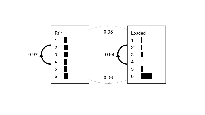
Figure 3: A simple HMM derived from the sequence of 300 dice rolls. As in Fig. 1, transition probabilities are shown as weighted lines and emission probabilities as horizontal grey bars.
This appears to be fairly close to the actual model, despite the fact that the training data consisted of just a single sequence. One would typically derive an HMM from a list of many such sequences (hence why the input argument is a list and not a vector) but this example is simplified for clarity.
Profile Hidden Markov Models
A profile hidden Markov model is an extension of a standard HMM, where the emission and transition probabilities are position specific. That is, they can change at each point along the sequence. These models typically have many more parameters than their simpler HMM counterparts, but can be very powerful for sequence analysis. The precursor to a profile HMM is normally a multiple sequence alignment. Each column in the alignment will often (but not always) be represented by one internal position or “module” in the model, with each module consisting of three states:
- a silent delete state that does not emit residues.
- an insert state with emission probabilities reflecting the background residue frequencies averaged over the entire alignment.
- a match state with emission probabilities reflecting the residue frequencies in the alignment column.
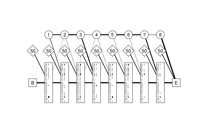
Figure 4 shows the three state types listed above as circles diamonds and rectangles, respectively. The states are linked by transition probabilities shown as weighted lines in the graph.
Consider this small partial alignment of amino acid sequences from Durbin et al (1998) chapter 5.3:
data(globins)
globins

##            [,1] [,2] [,3] [,4] [,5] [,6] [,7] [,8] [,9] [,10]
## HBA_HUMAN  "V"  "G"  "A"  "-"  "-"  "H"  "A"  "G"  "E"  "Y"
## HBB_HUMAN  "V"  "-"  "-"  "-"  "-"  "N"  "V"  "D"  "E"  "V"
## MYG_PHYCA  "V"  "E"  "A"  "-"  "-"  "D"  "V"  "A"  "G"  "H"
## GLB3_CHITP "V"  "K"  "G"  "-"  "-"  "-"  "-"  "-"  "-"  "D"
## GLB5_PETMA "V"  "Y"  "S"  "-"  "-"  "T"  "Y"  "E"  "T"  "S"
## LGB2_LUPLU "F"  "N"  "A"  "-"  "-"  "N"  "I"  "P"  "K"  "H"
## GLB1_GLYDI "I"  "A"  "G"  "A"  "D"  "N"  "G"  "A"  "G"  "V"
Position-specific patterns include a high probability of observing a “V”
at position 1 and an “A” or “G” at position 3. When tabulating the
frequencies it is also prudent to add pseudo-counts, since the absence
of a particular transition or emission type does not preclude the
possibility of it occurring in another (unobserved) sequence.
Pseudo-counts can be Laplacean (adds one of each emission and transition
type), background (adjusts the Laplacean pseudo-counts to reflect the
background frequencies derived from the entire alignment), or user
defined, which can include more complex pseudo-count schemes such as
Dirichlet mixtures (Durbin et al. 1998).
The default option for the derivePHMM function is “background”.
The following code derives a profile HMM from the globin data and plots the model:
globins.PHMM <- derivePHMM(globins, residues = "AMINO", seqweights = NULL)
plot(globins.PHMM)

Figure 4: Profile HMM derived from a partial globin sequence alignment. Match states are shown as rectangles, insert states as diamonds, and delete states as circles. Grey horizontal bars represent the emission probabilities for each residue in the alphabet (in this case the amino acid alphabet) at each position in the model. Numbers in the delete states are simply model module numbers, while those in the insert states are the probabilities of remaining in the current insert state at the next emission cycle. Lines are weighted and directed where necessary to reflect the transition probabilities between states. The large “B” and “E” labels represent are the silent begin and end states, respectively.
Note that there are only 8 internal modules (excluding the begin and end
states), while the alignment had 10 columns. The derivePHMM function
decided (using the maximum a posteriori algorithm) that there was not
enough residue information in columns 4 and 5 of the alignment to
warrant assigning them internal modules in the model. Instead, the last
sequence in the alignment (GLB1_GLYDI) was considered to have entered
the insert state at position 3 where it remained for two emission cycles
(emitting an “A” and a “D”) before transitioning to the match state in
module 4. We can show this by calculating the optimal path of that
sequence through the model, again using the Viterbi algorithm:
path <- Viterbi(globins.PHMM, globins["GLB1_GLYDI", ])$path
path

##  [1] 1 1 1 2 2 1 1 1 1 1
The “path” element of the Viterbi object is an integer vector with elements taking values 0 (“delete”), 1 (“match”) or 2 (“insert”). The path can be expressed more intuitively as characters instead of indices as follows:
c("D", "M", "I")[path + 1]

##  [1] "M" "M" "M" "I" "I" "M" "M" "M" "M" "M"
Note that the addition of 1 to each path element is simply to convert from the C/C++ indexing style (which begins at 0) to R’s style.
Sequences do not need to be aligned to produce a profile HMM. The
function derivePHMM can optionally take a list of unaligned sequences,
in which case the longest sequence is used as a ‘seed’ to create a
preliminary profile HMM, and the model is iteratively trained with the
sequence list using either the Baum Welch or Viterbi training algorithm
(see model training section below).
File I/O
Profile HMMs can be exported as text files in the HMMER v3 format
(http://www.hmmer.org/) using the function writePHMM. For example,
the small globin profile HMM can be exported by running
writePHMM(globins.PHMM). Similarly, a HMMER v3 text file can be parsed
into R as an object of class “PHMM” with the function readPHMM.
Sequence Simulation
To simulate data with random variation, the aphid package features
the function generate with methods for both HMMs and PHMM objects.
Sequences are generated recursively using the transition and emission
probabilities from within the model. There are two compulsory arguments,
a model (object class “HMM” or “PHMM”) and the “size” argument, which
specifies the maximum length of the sequence (this prevent an overflow
situation that can occur if insert-insert transition probabilities are
relatively high). For example, the following code simulates a list of 10
random sequences from the small globin profile HMM:
sim <- list(length = 10)
set.seed(9999)
for(i in 1:10) sim[[i]] <- generate(globins.PHMM, size = 20)
sim

## $length
##   M   M   M   M   I   I   M   M   M   M
## "N" "G" "T" "K" "K" "V" "H" "F" "G" "V"
##
## [[2]]
##   D   M   M   M   M   M   M   I   M
## "-" "N" "V" "N" "G" "P" "G" "V" "L"
##
## [[3]]
##   M   D   D   M   M   M   M   M
## "N" "-" "-" "H" "Y" "E" "V" "V"
##
## [[4]]
##   M   M   M   M   M   M   M   M
## "A" "W" "A" "N" "R" "P" "T" "G"
##
## [[5]]
##   M   M   M   M   M   M   M   M
## "G" "V" "A" "V" "E" "D" "T" "V"
##
## [[6]]
##   M   M   M   M   M   M   M   M
## "T" "G" "G" "Y" "A" "G" "S" "Y"
##
## [[7]]
##   M   M   M   M   M   M   I   M   M
## "I" "W" "A" "T" "A" "P" "K" "Y" "P"
##
## [[8]]
##   M   M   M   M   M   M   M   M
## "V" "N" "G" "D" "A" "G" "R" "Y"
##
## [[9]]
##   M   M   M   D   D   D   D   M
## "V" "N" "W" "-" "-" "-" "-" "H"
##
## [[10]]
##   D   D   D   M   M   M   M   M
## "-" "-" "-" "D" "K" "N" "A" "V"
Note that the names attributes specify which state each residue was emitted from, and gap symbols are emitted from delete states. If these gaps are not required they can be removed as follows:
sim <- lapply(sim, function(s) s[names(s) != "D"])
Model Training
The aphid package offers the function train for optimizing model
parameters using either the Baum Welch or Viterbi training algorithm.
Both are iterative refinement algorithms; the former does not rely on a
multiple sequence alignment but is generally much slower than the
latter. The Viterbi training operation can be sped up further on
multi-CPU machines by specifying the “cores” argument for parallel
processing. The best choice of training algorithm will generally depend
on the nature of the problem and the computing resources available. For
more information see Durbin et al (1998) chapter 3.3 for standard HMMs
and chapter 6.5 for profile HMMs.
The following code trains the small globin profile HMM with the sequences simulated in the previous step using the Baum Welch algorithm.
globins2.PHMM <- train(globins.PHMM, sim, method = "BaumWelch",
                       deltaLL = 0.01, seqweights = NULL)

## Iteration 1 log likelihood = -213.8818
## Iteration 2 log likelihood = -187.5671
## Iteration 3 log likelihood = -186.2003
## Iteration 4 log likelihood = -185.4684
## Iteration 5 log likelihood = -185.0501
## Iteration 6 log likelihood = -184.8302
## Iteration 7 log likelihood = -184.7419
## Iteration 8 log likelihood = -184.7162
## Iteration 9 log likelihood = -184.6974
## Iteration 10 log likelihood = -184.6543
## Iteration 11 log likelihood = -184.5744
## Iteration 12 log likelihood = -184.4634
## Iteration 13 log likelihood = -184.3386
## Iteration 14 log likelihood = -184.2147
## Iteration 15 log likelihood = -184.1037
## Iteration 16 log likelihood = -184.0166
## Iteration 17 log likelihood = -183.9569
## Iteration 18 log likelihood = -183.9197
## Iteration 19 log likelihood = -183.8976
## Iteration 20 log likelihood = -183.8846
## Iteration 21 log likelihood = -183.8769
## Convergence threshold reached after 21 EM iterations
As shown in the feedback (which can be switched off by setting “quiet = TRUE”), this operation took 7 expectation-maximization iterations to converge to the specified delta log-likelihood threshold of 0.01.
Sequence Alignment
The aphid package can be used to produce high-quality multiple
sequence alignments using the iterative model training method outlined
above. The function align takes as its primary argument a list of
sequences either as a “DNAbin” object, an “AAbin” object, or a list of
character sequences. An object of class “PHMM” can be passed to the
function as an optional secondary argument (“model”), in which case the
sequences are simply aligned to the model to produce the alignment
matrix. If “model” is NULL, a preliminary model is first derived using
the ‘seed’ sequence method outlined above, after which the model is
trained using either the Baum Welch or Viterbi training algorithm
(specified via the “method” argument). The sequences are then aligned
to the model in the usual fashion to produce the alignment. Note that if
only two sequences are present inthe input list, the align function
will perform a pairwise alignment without a profile HMM (Smith-Waterman
or Needleman-Wunch alignment).
In this final example, we will deconstruct the original globin alignment and re-align the sequences using the original PHMM as a guide.
globins <- unalign(globins)
align(globins, model = globins.PHMM, seqweights = NULL, residues = "AMINO")

##            1   2   3   I   I   4   5   6   7   8
## HBA_HUMAN  "V" "G" "A" "-" "-" "H" "A" "G" "E" "Y"
## HBB_HUMAN  "V" "-" "-" "-" "-" "N" "V" "D" "E" "V"
## MYG_PHYCA  "V" "E" "A" "-" "-" "D" "V" "A" "G" "H"
## GLB3_CHITP "V" "K" "G" "-" "-" "-" "-" "-" "-" "D"
## GLB5_PETMA "V" "Y" "S" "-" "-" "T" "Y" "E" "T" "S"
## LGB2_LUPLU "F" "N" "A" "-" "-" "N" "I" "P" "K" "H"
## GLB1_GLYDI "I" "A" "G" "A" "D" "N" "G" "A" "G" "V"
Note that the column names show the progressive positions along the model and where residues were predicted to have been emitted by insert states (e.g. the 4th and 5th residues of sequence 7).
Further Reading
This package was written based on the algorithms described in Durbin et al (1998). This book offers an in depth explanation of hidden Markov models and profile HMMs for users of all levels of familiarity. Many of the examples and datasets in the package are directly derived from the text, which serves as a useful primer for this package. There are also excellent resources available for those wishing to use profile HMMs outside of the R environment. The aphid package maintains compatibility with the HMMER software suite through the file input and output functions readPHMM and writePHMM. Those interested are further encouraged to check out the SAM software package, which also features a comprehensive suite of functions and tutorials.
Acknowledgements
This software was developed at Victoria University of Wellington, NZ, with funding from a Rutherford Foundation Postdoctoral Research Fellowship award from the Royal Society of New Zealand.
References
Durbin, Richard, Sean Eddy, Anders Krogh, and Graeme Mitchison. 1998. Biological Sequence Analysis: Probabilistic Models of Proteins and Nucleic Acids. Cambridge: Cambridge University Press.
Eddelbuettel, Dirk, and Romain Francois. 2011. “Rcpp: seamless R and C++ integration.” Journal of Statistical Software 40 (8): 1–18. http://www.jstatsoft.org/v40/i08/.
Ooms, Jeroen. 2016. openssl: toolkit for encryption, signatures and certificates based on OpenSSL. R package. https://cran.r-project.org/package=openssl.
Paradis, Emmanuel. 2012. Analysis of Phylogenetics and Evolution with R. Second Edi. New York: Springer.
Paradis, Emmanuel, Julien Claude, and Korbinian Strimmer. 2004. “APE: analyses of phylogenetics and evolution in R language.” Bioinformatics 20: 289–90. doi:10.1093/bioinformatics/btg412.
R Core Team. 2017. “R: A Language and Environment for Statistical Computing.” Vienna, Austria: R Foundation for Statistical Computing. https://cran.r-project.org/.